HTDYM (How To Deploy Your Model)

This post assumes a Scaling Book skim’s worth of familiarity with topics in LLM inference.

We have a motto at Sail: there are no bad chips, only bad prices. Buying the hardware everyone else overlooks is a big part of how we maximize intelligence-per-dollar. A chip doesn’t have to be perfectly ideal for a workload to be worth using, just underpriced for how it performs there. For every model we serve, we want to know exactly what every chip on the market is worth to us.

That question is not as simple as “which chip has the most FLOPs.” Models come in all different shapes and sizes: some are MoE, some are dense; some have been trained to run in MXFP8, while others must be run in full BF16 precision; some have compressed attention mechanisms while others alternate sliding window and dense attention. Workloads for a given model can differ just as much: prefill is compute-bound, while decode is typically dominated by memory bandwidth, so a chip with a high ratio of memory bandwidth to FLOPs can be a great decode chip and a mediocre prefill chip, and with disaggregated serving, nothing forces us to run both phases on the same hardware. And even once the model, workload, and chip are all fixed, how the model is sharded over the chips can change tokens per dollar by >3x, a dimension of the problem we’ve found to be consistently underrated.

Today, we’re open sourcing HTDYM (How To Deploy Your Model), our internal performance modeling infrastructure that helps us make these deployment decisions at scale.

The code is available at github.com/sailresearchco/htdym, and you can play around with a hosted version of our UI for it at htdym.sailresearch.com.

Benchmarking

You may be asking: can’t you just solve this with benchmarking? Just spin up vLLM/SGLang on each hardware platform we’re considering serving on, grid search over its parallelism and batching knobs, measure tok/s and read off the winner? This is the approach of SemiAnalysis’ InferenceX platform, and we do plenty of this ourselves as well, but benchmarking alone has some major problems.

• We can’t benchmark what we don’t have. We often want to evaluate hardware that is not widely available yet, or in unpopular configurations that haven’t been publicly benchmarked.
• Large search space. Evaluating every combination of shardings × placements × batch sizes × workload shapes, per model, per machine configuration, can become time consuming very quickly. We’d like to get answers in seconds or minutes instead of days or weeks.
• Engine performance ≠ Achievable performance. A benchmark measures the particular engine’s implementation as much as the hardware. This is a massive problem. Because inference engines have to support so many models (often on day 0!), there is frequently a large gap between an engine’s out-of-the-box performance and the performance achievable with additional kernel optimization / tuning. This bites especially hard with more niche hardware platforms, which are often relatively neglected. An under-optimized engine implementation can also mislead us about the best sharding for the model on a given chip. E.g. if the engine’s kernels or communication overlap happen to be poor at, say, TP=4/EP=4, the benchmark can make it seem like that sharding is bad, when in reality the implementation is bad, and that configuration may be exactly what the hardware runs best.

Ideally, we want a system that prices each model and sharding based on the hardware’s capabilities, independent of software maturity. This keeps us from writing off good shardings (and good chips) because of immature kernels, and if a real benchmark lands far below the estimated ceiling it can help us diagnose where to target kernel work.

Rooflines

Before we can think about which hardware runs a model best, it’s useful to think about how to determine the expected performance of a model on arbitrary hardware at all. Roofline modeling enables us to determine an upper bound on the performance of a model on a given chip using only simple math.

At the highest level, we just calculate how many floating point operations our workload requires and how many bytes it loads from memory, and then divide each of them by the rate the hardware can do them at. Taking the max of the two gives us an upper bound which assumes perfect overlap of compute and data movement, while the sum gives us an upper bound assuming no such overlap.

When working with multiple chips, we have to account for a third resource: the network. To serve large models, we almost always must shard them over multiple chips because their weights are too large to fit in the memory of a single accelerator. Each way of sharding a model imposes different communication requirements between chips at various points in the forward pass, but as with the other resources, we can simplify this down to bytes moved divided by network bandwidth:

Our revised roofline bounds are thus:

There is a lot more nuance to using roofline models effectively, and to thinking about LLM inference in general, than we have space for here. I highly recommend How To Scale Your Model¹ (“the Scaling Book”) for more.

So can we answer “what hardware should run this model?” with the formula above? Not yet. Rooflines on their own have a couple of issues:

• Many of the roofline’s inputs are difficult to know a priori. “Bytes moved” is not a property of the model or hardware, it depends almost entirely on how we choose to shard it, and it’s often non-obvious how to shard a model on a given hardware/topology.² Even bytes loaded depends on the sharding: under expert parallelism a chip only streams the experts its tokens activated that step, and a tensor parallelism degree that exceeds a model’s KV head count can require replicating heads.
• Rooflines bake in homogeneity assumptions that break down in the real world.
  • Aggregating FLOPs across operations loses key detail on the size of each operation. This is increasingly important on modern hardware, where large operand sizes are required to get maximum throughput out of increasingly large and heavily pipelined matrix units.
  • Models mix floating point formats across their architecture. Attention and router ops may be done in BF16 while expert computation is done in MXFP8, etc., each at different hardware rates.
  • Not all “bytes moved” are equal. Collectives differ in their pattern of communication, even when the byte counts match. For example, all-gather and all-reduce run efficiently on torus topologies while all-to-all collectives run poorly on them.
• A roofline doesn’t know what fits. Weights must fit in HBM, and whatever room is left over holds the KV cache, which caps the max batch size, and in decode, batch size is critical for determining performance via amortization. A chip that looks great on the roofline may not be able to hold enough sequences to reach it.

HTDYM solves these issues by carefully computing rooflines per-op, and searching over all possible sharding configurations to select the best one. Unlike inference simulators (e.g. Vidur), it estimates achievable performance from hardware capabilities rather than simulating a particular inference engine, and unlike a simple roofline calculator (e.g. LLM-Viewer) it accounts for inter-chip communication costs and automatically selects the best sharding.

Pricing

HTDYM’s pricing engine takes five inputs:

• A model: an ordered list of layers, each with an attention config (MHA, GQA, MLA), FFN config (dense, MoE), and per-tensor float precisions.
• Hardware: the specs for a chip/group of chips, e.g. peak matmul rates per format, HBM capacity/bandwidth, and interconnect specs.
• A sharding: the degree of tensor parallelism, data parallelism, expert parallelism, expert tensor parallelism, and pipeline parallelism to shard the model over the chips with.
• A workload: prefill or decode, input and output lengths, and a batch size.³
• A “cost backend”: a set of functions used to estimate the cost of operations.

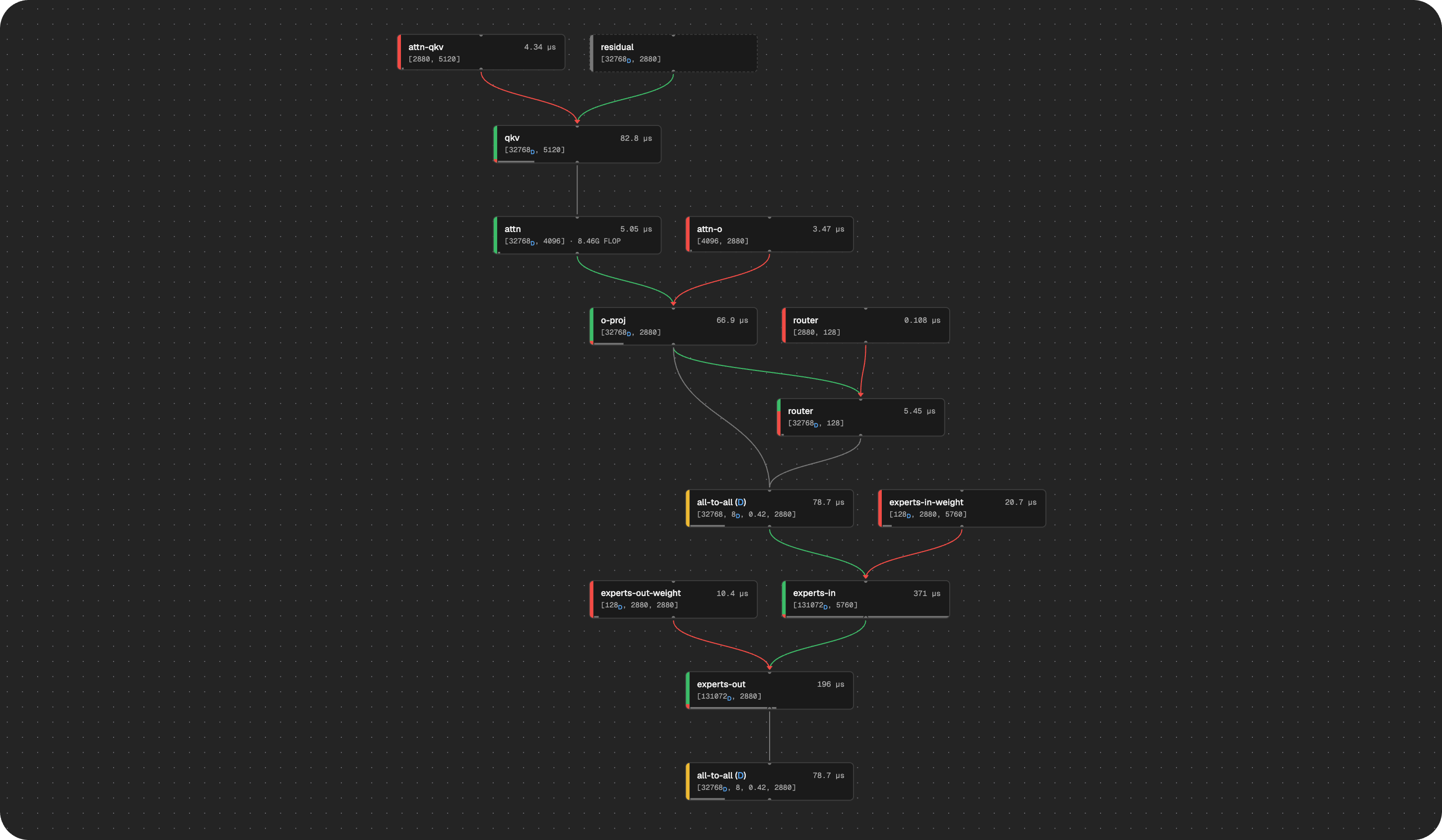
From these inputs, the engine works like a compiler, “lowering” the model into a DAG of operations: GEMMs with their actual sharded shapes, attention ops with their per-chip KV traffic, weight loads, and placeholders for collectives depending on the sharding (more on this below).

The engine then makes two passes over this DAG. First, collective placeholders are resolved into concrete collectives (all-gather, all-to-all, all-reduce, etc.). Then, the cost backend is fed the resolved DAG and returns the estimated total and per-op time for the workload.⁴ Combined with what we actually pay per chip-hour, time per input/output token becomes input/output tokens per dollar. We’ve found it useful to compare and quote these numbers relative to a “minimum viable H100 setup” (HMVP for short), the best sharding for the given workload on the smallest H100 machine which can fit the model.⁵

Resolving Collectives

Why placeholders? Because the best set of collectives to get from one sharding to another is not always obvious. Here’s an example: suppose every chip along some axis of a device mesh holds a partial sum of the same tensor, and we need every chip to end up with the full, summed-up tensor. This is a common situation after a sharded matmul, e.g. the output of a tensor-parallel MLP layer.

Borrowing notation from the Scaling Book: A[I_X, J] denotes a tensor A with its I dimension sharded over mesh axis X, and {U_X} marks tensors that are unreduced partial sums pending a reduction over X. So our problem is getting from A[I, J] {U_X} to A[I, J].

On a ring topology, the obvious plan is a single AllReduce_X, which moves roughly 2|A| bytes per chip. But if another mesh axis Y is idle, we can do something clever. Reduce a smaller tensor by first sharding A over Y, then gather the shards back at the end.

The slice step is free, each chip simply keeps only its 1/|Y| slice of its local partial sums and throws away the rest. The AllReduce_X then moves only 2|A|/|Y| bytes per chip, and the AllGather_Y moves approximately |A| bytes, thus a total of roughly |A|(1 + 2/|Y|), which beats the single AllReduce_X whenever |Y| > 2.

Hand-coding tricks like this quickly becomes a nightmare, so instead HTDYM solves this like a shortest path search problem. Nodes are shardings, edges are collectives, and edge weights are the cost backend’s prices for them. Clever plans like the above then fall out of a search over this graph instead of being special-cased, and because the edge weights come from the cost backend, higher fidelity backends also improve collective resolution.

Cost Backends

Currently, the only implemented backend is a per-op roofline-style backend, which prices each op according to its type. GEMMs take FLOPs / Hardware FLOP/s time (using the correct spec sheet numbers for the data type of the GEMM), weight loads take Bytes / HBM Bandwidth/s time, etc. Collectives are priced using both a per-hardware latency and bandwidth term.

We apply a configurable blanket derating to these bandwidth and FLOP numbers based on the chip, as in practice many vendors (some more than others!) quote spec sheet numbers that are unrealistic in real workloads. For GEMMs, we apply a special derating depending on the size of the matrices involved if they fall below the estimated tile size of the chip’s matmul units.

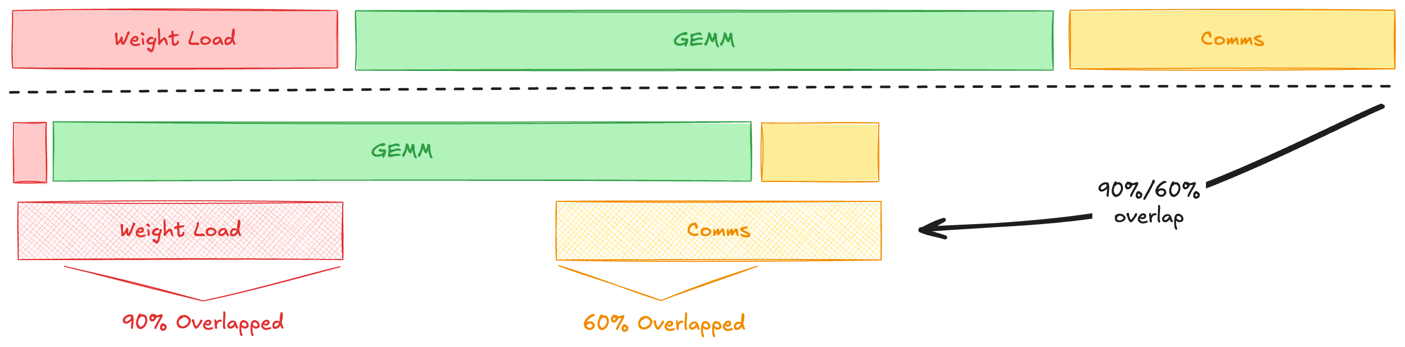
The backend then combines these per-op costs into an end-to-end estimate. This step is configurable by the user: for each non-compute resource (memory, communication), the user specifies what fraction of that resource’s time can be overlapped with / hidden behind compute. The remainder is exposed, and will extend the total time. For example, with 90% memory overlap and 60% comms overlap, only 10% of the total weight-load time and 40% of the total communication time are exposed, and (given enough compute to hide behind) the estimate becomes:

The fact that cost backends are pluggable makes HTDYM more flexible than just a roofline calculator, as its DAG representation and lowering machinery can be reused no matter how the cost backend is implemented. In the future, we may implement other, more sophisticated cost backends depending on our needs, e.g. a backend which uses dependencies from the DAG to determine possible overlap, a high fidelity hardware simulator backend, a backend which interpolates real world measurements of different operations on a given hardware platform, etc.

Search

Now that we have a good cost oracle (the pricing engine), the question of “what hardware” and “what sharding” becomes a search problem.

For a given model and machine, HTDYM enumerates every valid sharding configuration (factorizations of the chip count into PP × TP × DPA × EP × ETP⁶), every placement of those roles onto the physical axes of the machine,⁷ and (when required) every MoE dispatch strategy.

Each candidate is checked for feasibility before it’s priced (the weights fit, sufficient KVs fit, etc.). When estimating decode performance, users specify a “serving policy” that determines the batch size (throughput-focused = fill KV capacity when only throughput matters, interactivity-focused = largest batch that still meets a tok/s/user requirement). Candidates are checked in parallel and ranked by tokens per dollar relative to an HMVP baseline (the best sharding on the smallest H100 setup that fits the model).

Running this search across the catalog of chips we have liquidity for is how we put the “no bad chips” thesis into practice. When we priced Gemma 4 31B across 24 chips in 3455 configurations, we identified that by serving on TPU v6e, we could achieve a ~3x input token cost reduction at only a ~25% decode token cost increase vs. our current H200 setup. Given our typically prefill-heavy workload for Gemma 4 31B, this is the exact kind of tradeoff we are eager to make. After some kernel work, we’ve been able to achieve 87.5% of HTDYM’s estimated prefill performance⁸ in the real world with v6e. We’re now shifting much of our Gemma traffic to the TPU, and will have more to share here soon.

For large topologies, this kind of exhaustive search can be quite expensive. We’re happy enough with its performance given the current topology sizes we work with (≤64 chips), but as scale-up domain sizes continue to grow (looking at you NVL1152...), we’ll need to implement heuristics to prune the search space.

Caveats

As discussed in the cost backends section, our current primary cost backend is deliberately naive: it sums each resource over the op graph and combines the sums with tunable overlap fractions, but does not consider any lower-level hardware scheduling constraints that could affect the viability of this overlap, etc. It also relies on some rough per-chip fudge factors (“realizable FLOPs / HBM BW”) that we haven’t measured carefully.

In practice, for chip/model pairs we’ve studied closely, with reasonable overlap assumptions, HTDYM’s estimated performance is close to what we see in the real world with highly tuned implementations. This, of course, does not rule out bugs in models and hardware we haven’t looked closely at. Please file an issue if you spot any suspicious results.

There are also several aspects of real-world serving that HTDYM does not currently model. The engine prices a single static batch size per workload, while real engines run continuous batching, with sequences joining and leaving the batch every step (and, except under disaggregation, mixed prefill/decode steps). Relatedly, while we price prefill and decode independently, we do not yet model the cost of KV cache transfer between prefill and decode pools in disagg setups. For most interconnects and workload shapes this is small relative to compute, but it is not free, and it can matter a lot when the pools have poor interconnect between them. Speculative decoding and expert imbalance in MoE routing are also currently unmodeled, but we plan to add support for incorporating them into HTDYM’s estimates in the future.

Finally, to state the obvious: per-op rooflines assume the hardware is always doing useful work. In reality, kernel launch latency, CPU bottlenecks, and other fixed overheads can begin to dominate at small batch sizes (on some platforms more than others), and our estimates will be most optimistic in these cases. Sail is focused on achieving maximum efficiency, which means we built HTDYM around modeling large, steady-state, throughput-focused workloads. Treat its numbers for small-batch, latency-sensitive configurations as much looser upper bounds.

Conclusion

There are arbitrages everywhere for those with the eyes to see and the tools to model performance properly. The gap between the most and least efficient way to run our models on the accelerators available to us is huge, and is constantly changing as prices and our workloads do. Having infrastructure that helps us price and plan deployments quickly helps keep Sail afloat in a sea of hardware options.

Try it out yourself at htdym.sailresearch.com, and/or contribute on GitHub. And if this kind of work excites you, we’re hiring.